Step-by-step guide for analysis of H&E-stained imaging data
This tutorial will guide you through the process of running SpaHDmap on your data. Our example data is the 10X Visium ST dataset MPBS-01 sequenced from an adult mouse brain posterior section comprising a H&E image, we will take the H&E image and the spot expression data as input to run SpaHDmap. This data could be downloaded from 10X Genomics or Google Drive.
1. Import necessary libraries
Please make sure you have installed SpaHDmap.
!pip install SpaHDmap
[1]:
import torch
import numpy as np
import scanpy as sc

import SpaHDmap as hdmap
/home/qk/anaconda3/lib/python3.11/importlib/__init__.py:126: FutureWarning: The legacy Dask DataFrame implementation is deprecated and will be removed in a future version. Set the configuration option `dataframe.query-planning` to `True` or None to enable the new Dask Dataframe implementation and silence this warning.
  return _bootstrap._gcd_import(name[level:], package, level)
2. Set the parameters and paths
In this section, we will set the parameters and paths for the SpaHDmap model, including:
Parameters:
rank: the rank / number of components of SpaHDmap modelseed: the random seedverbose: whether to print the log information
Paths:
root_path: the root path of the experimentproject: the name of the projectresults_path: the path to save the results
Parameters settings
By default, we set the rank to 20, the seed to 123, and the verbose to True. You can modify the parameters according to your data.
[3]:
rank = 20
seed = 123
verbose = True

np.random.seed(seed)
torch.manual_seed(seed)
[3]:
<torch._C.Generator at 0x7f700817e570>
Paths settings
These paths are set with respect to the current directory. You can modify the paths according to your data.
[4]:
root_path = '../experiments/'
project = 'MPBS01'

results_path = f'{root_path}/{project}/Results_Rank{rank}/'
3. Load the data and pre-process
The data used in this tutorial is a 10X Visium ST dataset MPBS-01 sequenced from an adult mouse brain sagittal section, could be downloaded from 10X Genomics or Google Drive.
You are able to utilize the function prepare_stdata for data loading and pre-precessing. This function supports loading data in two ways: directly loading an Anndata object or loading from file paths. There are several essential parameters, as follows:
section_name: The name designating the section.image_path: The location path of the image.scale_rate: The scaling ratio applied to the input images. The default value is 1.create_mask: Whether to create a mask for the image. The default value is True.swap_coord: A parameter indicating whether to swap the row and column coordinates. The default value is True.
For more details of this function, please refer to the API document!
Load data with an Anndata object
We recommend to download / load the Anndata object using the api sc.datasets.visium_sge from scanpy, and set include_hires_tiff=True to download the hires image.
In this case, this data will be saved locally in the folder data/id_of_the_section, and next time you can load the data from the local folder.
[6]:
section_id = 'V1_Mouse_Brain_Sagittal_Posterior'

# Download the data from the 10X website (set include_hires_tiff=True to download the hires image)
adata = sc.datasets.visium_sge(section_id, include_hires_tiff=True)
image_path = adata.uns["spatial"][section_id]["metadata"]["source_image_path"]

# or load the data from a local folder
# adata = sc.read_visium(f'data/{section_id}', count_file='filtered_feature_bc_matrix.h5')
# image_path = f'data/{section_id}/image.tif'
/tmp/ipykernel_1835111/175887311.py:4: FutureWarning: Use `squidpy.datasets.visium` instead.
  adata = sc.datasets.visium_sge(section_id, include_hires_tiff=True)
/home/qk/anaconda3/lib/python3.11/site-packages/scanpy/datasets/_datasets.py:555: FutureWarning: Use `squidpy.read.visium` instead.
  return read_visium(sample_dir, source_image_path=source_image_path)
/home/qk/anaconda3/lib/python3.11/site-packages/anndata/_core/anndata.py:1820: UserWarning: Variable names are not unique. To make them unique, call `.var_names_make_unique`.
  utils.warn_names_duplicates("var")
/home/qk/anaconda3/lib/python3.11/site-packages/anndata/_core/anndata.py:1820: UserWarning: Variable names are not unique. To make them unique, call `.var_names_make_unique`.
  utils.warn_names_duplicates("var")
Then we are able to load and pre-process the data using function prepare_stdata, which will normalize both the gene expression and the image. Note that it will be fine if you provide an adata object whose expression data has already been normalized (but should not be scaled, the expression data has to be non-negative), this function will recognize the normalized expression data automatically.
Subsequently, we will utilize the function select_svgs to select spatial variable genes (SVGs). By default, it will identify 3,000 SVGs in accordance with the Moran’s I index. Alternatively, you may set method='sparkx' or method='bsp' to identify SVGs based on the SPARK-X or BSP methods respectively.
[7]:
# Load the data from the 10X Visium folder
mouse_posterior = hdmap.prepare_stdata(adata=adata,
                                       section_name='mouse_posterior',
                                       image_path=image_path,
                                       scale_rate=1)

hdmap.select_svgs(mouse_posterior, n_top_genes=3000, method='moran')
*** Reading and preparing AnnData for section mouse_posterior ***
Spot radius found in AnnData: 45
Pre-processing gene expression data for 3355 spots and 32285 genes.
Swapping x and y coordinates.
Processing image, seems to be HE image.
Selected 3000 SVGs using moran method.
prepare_stdata returns a STData object, which contains several key attributes for the analysis:
.adata: An AnnData object holding the normalized gene expression data and spot metadata.
.image: A NumPy array of the high-resolution tissue image.
.spot_coord: The spatial coordinates for each spot.
.radius and .scale_rate: Metadata defining the spot size and image scaling.
.scores: An empty dictionary that will be populated with analysis results (e.g., NMF, SpaHDmap scores).”
[8]:
mouse_posterior
[8]:
STData object for section: mouse_posterior
Number of spots: 3355
Number of genes: 3000
Image shape: (3, 11607, 11620)
Scale rate: 1
Spot radius: 45
Image type: HE
Available scores:
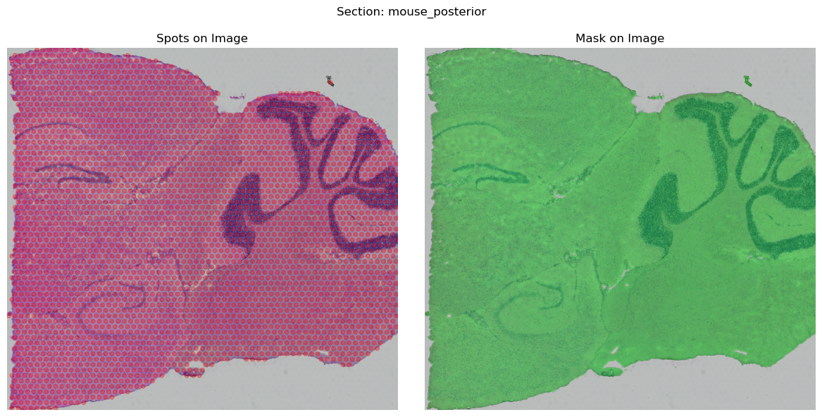
You may use the function .show() to display the processed STData. If there is a mismatch between the spots and the image, it may be necessary for you to set swap_coord=False or handle the coordinate processing independently.
[8]:
mouse_posterior.show()
Load data from file paths
Alternatively, you can load the data by providing the paths of spot coordinates, gene expression and image. In this case, you have to provide the radius, which is the radius of each spot measured in pixels on the original high-resolution image.
These data can be downloaded from the 10X Genomics website in:
spot coordinates:
Output and supplemental files -> Spatial imaging data -> tissue_positions_list.csv, please make sure that the first column is the spot names and the last two columns are the coordinates.gene expression:
Output and supplemental files -> Feature / barcode matrix (both filtered and raw are fine), a hdf5 file or a csv file with the first row as the gene names and the first column as the spot names.image:
Input files -> Image (TIFF).
Then you can load and pre-process the data using the following code:
[ ]:
# Load the data from file paths
mouse_posterior = hdmap.prepare_stdata(section_name='mouse_posterior',
                                       image_path='data/V1_Mouse_Brain_Sagittal_Posterior/image.tif',
                                       spot_coord_path='data/V1_Mouse_Brain_Sagittal_Posterior/spatial/tissue_positions_list.csv',
                                       spot_exp_path='data/V1_Mouse_Brain_Sagittal_Posterior/filtered_feature_bc_matrix.h5',
                                       scale_rate=1,
                                       radius=45) # Has to be provided if load from file paths

hdmap.select_svgs(mouse_posterior, n_top_genes=3000, method='moran')
[10]:
mouse_posterior
[10]:
STData object for section: mouse_posterior
Number of spots: 3355
Number of genes: 3000
Image shape: (3, 11607, 11620)
Scale rate: 1
Spot radius: 45
Image type: HE
Available scores:
Visualize the spots with image
4. Run SpaHDmap
To run SpaHDmap, we need to initialize the Mapper object, which contains the following attributes:
section: the section objectresults_path: the path to save the resultsrank: the rank / number of components of the NMF model, default is 20reference: dictionary to assign the reference section for each query section, default is None (only for multi-sections)ratio_pseudo_spots: ratio of pseudo spots to sequenced spots, default is 5verbose: whether to print the log information, default is True
[12]:
# Initialize the SpaHDmap runner
mapper = hdmap.Mapper(mouse_posterior, results_path=results_path, rank=rank, verbose=verbose)
*** Preparing the tissue splits and creating pseudo spots... ***
*** Single section detected. Using its 3000 genes. ***
*** The split size is set to 256 pixels. ***
For section mouse_posterior, divide the tissue into 1410 sub-tissues, and create 15000 pseudo spots.
*** Using GPU ***
Run all steps in one function
We can run all steps in one function run_SpaHDmap after obtaining the Mapper object.
[13]:
# Run all steps in one function
mapper.run_SpaHDmap(save_score=False, save_model=True, load_model=True, visualize=True, format='png')

# If you want to lower the GPU memory usage, you can set `batch_size` to a smaller number
# mapper.args.batch_size = 16 (default 32)
# mapper.run_SpaHDmap(save_score=False, save_model=True, visualize=False)
Step 1: Run NMF
*** Performing NMF... ***
*** Visualizing and saving the embeddings of NMF... ***
Step 2: Pre-train the SpaHDmap model
/home/qk/projects/DeepFuseNMF/SpaHDmap/train.py:528: FutureWarning: `torch.cuda.amp.GradScaler(args...)` is deprecated. Please use `torch.amp.GradScaler('cuda', args...)` instead.
  self.scaler = torch.cuda.amp.GradScaler()
/home/qk/projects/DeepFuseNMF/SpaHDmap/train.py:574: FutureWarning: `torch.cuda.amp.autocast(args...)` is deprecated. Please use `torch.amp.autocast('cuda', args...)` instead.
  with torch.cuda.amp.autocast():
[Iter: 200 / 5000], Epoch: 5, Loss: 0.045296, Learning rate: 3.984269e-04
[Iter: 400 / 5000], Epoch: 9, Loss: 0.001389, Learning rate: 3.937323e-04
[Iter: 600 / 5000], Epoch: 14, Loss: 0.000800, Learning rate: 3.859904e-04
[Iter: 800 / 5000], Epoch: 18, Loss: 0.000533, Learning rate: 3.753232e-04
[Iter: 1000 / 5000], Epoch: 23, Loss: 0.000433, Learning rate: 3.618989e-04
[Iter: 1200 / 5000], Epoch: 27, Loss: 0.000349, Learning rate: 3.459292e-04
[Iter: 1400 / 5000], Epoch: 32, Loss: 0.000305, Learning rate: 3.276661e-04
[Iter: 1600 / 5000], Epoch: 36, Loss: 0.000263, Learning rate: 3.073974e-04
[Iter: 1800 / 5000], Epoch: 40, Loss: 0.000240, Learning rate: 2.854430e-04
[Iter: 2000 / 5000], Epoch: 45, Loss: 0.000204, Learning rate: 2.621489e-04
[Iter: 2200 / 5000], Epoch: 49, Loss: 0.000186, Learning rate: 2.378826e-04
[Iter: 2400 / 5000], Epoch: 54, Loss: 0.000177, Learning rate: 2.130267e-04
[Iter: 2600 / 5000], Epoch: 58, Loss: 0.000166, Learning rate: 1.879733e-04
[Iter: 2800 / 5000], Epoch: 63, Loss: 0.000151, Learning rate: 1.631174e-04
[Iter: 3000 / 5000], Epoch: 67, Loss: 0.000142, Learning rate: 1.388511e-04
[Iter: 3200 / 5000], Epoch: 72, Loss: 0.000137, Learning rate: 1.155570e-04
Reached convergence, stop early
*** Finished pre-training the SpaHDmap model and saved at ../experiments//MPBS01/Results_Rank20//models//pretrained_model.pth ***
Step 3: Train the GCN model
*** Performing GCN... ***
*** Training GCN for mouse_posterior... ***
[Iter: 200 / 5000], Loss: 0.020134, Learning rate: 4.985215e-03
[Iter: 400 / 5000], Loss: 0.005996, Learning rate: 4.941093e-03
[Iter: 600 / 5000], Loss: 0.005459, Learning rate: 4.868331e-03
[Iter: 800 / 5000], Loss: 0.005296, Learning rate: 4.768075e-03
[Iter: 1000 / 5000], Loss: 0.005204, Learning rate: 4.641907e-03
[Iter: 1200 / 5000], Loss: 0.005148, Learning rate: 4.491816e-03
[Iter: 1400 / 5000], Loss: 0.005113, Learning rate: 4.320170e-03
[Iter: 1600 / 5000], Loss: 0.005087, Learning rate: 4.129675e-03
[Iter: 1800 / 5000], Loss: 0.005064, Learning rate: 3.923336e-03
[Iter: 2000 / 5000], Loss: 0.005046, Learning rate: 3.704407e-03
[Iter: 2200 / 5000], Loss: 0.005028, Learning rate: 3.476340e-03
[Iter: 2400 / 5000], Loss: 0.005014, Learning rate: 3.242732e-03
[Iter: 2600 / 5000], Loss: 0.005000, Learning rate: 3.007268e-03
[Iter: 2800 / 5000], Loss: 0.004988, Learning rate: 2.773660e-03
[Iter: 3000 / 5000], Loss: 0.004977, Learning rate: 2.545593e-03
[Iter: 3200 / 5000], Loss: 0.004966, Learning rate: 2.326664e-03
[Iter: 3400 / 5000], Loss: 0.004956, Learning rate: 2.120325e-03
[Iter: 3600 / 5000], Loss: 0.004947, Learning rate: 1.929830e-03
[Iter: 3800 / 5000], Loss: 0.004940, Learning rate: 1.758184e-03
[Iter: 4000 / 5000], Loss: 0.004934, Learning rate: 1.608093e-03
[Iter: 4200 / 5000], Loss: 0.004929, Learning rate: 1.481925e-03
[Iter: 4400 / 5000], Loss: 0.004924, Learning rate: 1.381669e-03
[Iter: 4600 / 5000], Loss: 0.004919, Learning rate: 1.308907e-03
[Iter: 4800 / 5000], Loss: 0.004914, Learning rate: 1.264785e-03
[Iter: 5000 / 5000], Loss: 0.004910, Learning rate: 1.250000e-03
*** Visualizing and saving the embeddings of GCN... ***
Step 4: Run Voronoi Diagram
Step 5: Train the SpaHDmap model
*** Training the model... ***
[Iter: 200 / 2000], Epoch: 5,Image Loss: 0.015830, Expression Loss: 0.499526, Total Loss: 0.179876,Learning rate: 4.522638e-03
[Iter: 400 / 2000], Epoch: 9,Image Loss: 0.005290, Expression Loss: 0.499479, Total Loss: 0.169933,Learning rate: 3.272888e-03
[Iter: 600 / 2000], Epoch: 14,Image Loss: 0.004265, Expression Loss: 0.498252, Total Loss: 0.168383,Learning rate: 1.728112e-03
[Iter: 800 / 2000], Epoch: 18,Image Loss: 0.003861, Expression Loss: 0.499170, Total Loss: 0.168273,Learning rate: 4.783620e-04
[Iter: 1000 / 2000], Epoch: 23,Image Loss: 0.003704, Expression Loss: 0.498331, Total Loss: 0.167820,Learning rate: 1.000000e-06
[Iter: 1200 / 2000], Epoch: 27,Image Loss: 0.003869, Expression Loss: 0.499399, Total Loss: 0.168879,Learning rate: 3.719031e-04
[Iter: 1400 / 2000], Epoch: 32,Image Loss: 0.003526, Expression Loss: 0.499157, Total Loss: 0.168087,Learning rate: 2.749663e-04
[Iter: 1600 / 2000], Epoch: 36,Image Loss: 0.003367, Expression Loss: 0.497708, Total Loss: 0.167496,Learning rate: 1.475598e-04
[Iter: 1800 / 2000], Epoch: 40,Image Loss: 0.003273, Expression Loss: 0.496405, Total Loss: 0.166965,Learning rate: 4.181507e-05
[Iter: 2000 / 2000], Epoch: 45,Image Loss: 0.003250, Expression Loss: 0.498291, Total Loss: 0.167455,Learning rate: 1.000000e-06
*** Finished training the SpaHDmap model and saved at ../experiments//MPBS01/Results_Rank20//models//trained_model.pth ***
*** Extracting SpaHDmap scores for mouse_posterior... ***
*** Visualizing and saving the embeddings of SpaHDmap... ***
Parameters of run_SpaHDmap are as follows:
save_score: whether to save the embeddings, default is Falsesave_model: whether to save the model, default is Trueload_model: whether to load the model if it has been trained and saved, default is Truevisualize: whether to visualize the results, default is Trueformat: the format of the visualization, default is ‘png’use_ann: whether to use Approximate Nearest Neighbors (ANN) for neighbor search, default is False
Note: For large dataset, we recommend setting use_ann=True for faster performance.
Run SpaHDmap step by step
Alternatively, you can run each step separately as follows to get a detailed understanding of the SpaHDmap model.
Run NMF to get the initial spot score and loading matrix
We need to run NMF on the gene expression data to get the initial spot score and loading matrix (metagene).
If save_score=True (default False), the NMF score will be saved in results_path/section_name/NMF/NMF_score.npy.
The loading matrix will be saved in results_path/V_para_NMF.csv
[14]:
# Run NMF on the gene expression data
mapper.get_NMF_score(save_score=False)

print(mouse_posterior.scores['NMF'].shape)
*** Using existing metagene for transfer learning... ***
(3355, 20)
We can visualize the NMF score for a specific index, sections can be the section or the name of the section or None.
In this case, we visualize the NMF score for the section ‘mouse_posterior’ and the index 2.
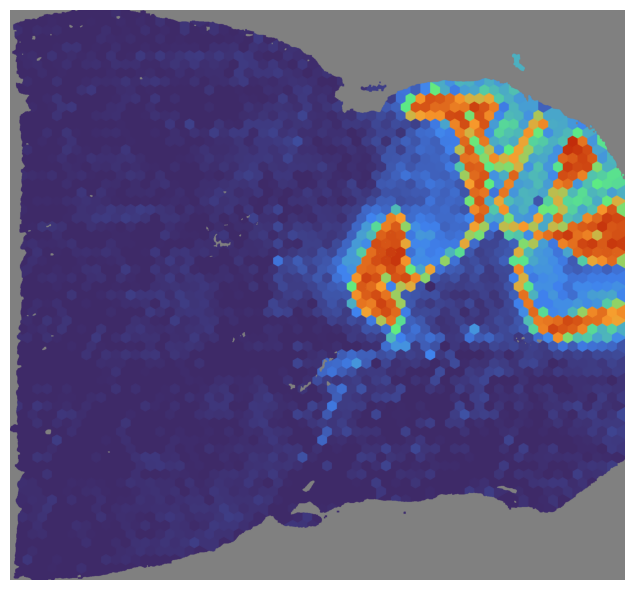
[15]:
mapper.visualize(mouse_posterior, use_score='NMF', index=2)
# mapper.visualize('mouse_posterior', use_score='NMF', index=2) # visualize given the name
# mapper.visualize(use_score='NMF', index=2) # ignore the section name if only one section
*** Visualizing and saving the embeddings of NMF... ***
Also, we can visualize without specifying the index, all NMF scores will be saved in results_path/section_name/NMF.
[16]:
# Save all NMF scores into `results_path/section_name/NMF`
mapper.visualize(use_score='NMF', format='png') # default is 'png'
*** Visualizing and saving the embeddings of NMF... ***
Pre-train the SpaHDmap model
In this step, we pre-train the SpaHDmap model based on the image prediction to get the sub-image embedding, which will be used to create the graph between spots, and used as the initial parameters for later training.
If save_model=True (default True), the pre-trained model will be saved in {results_path}/models/pretrain_model.pth
[17]:
# Pre-train the SpaHDmap model via reconstructing the HE image
mapper.pretrain(save_model=True)
*** Pre-trained model found at ../experiments//MPBS01/Results_Rank20//models//pretrained_model.pth, loading... ***
Train GCN to get smoothness score for sequenced and pseudo spots
In this step, we construct a graph on the basis of the spot coordinates and the sub-image embeddings. An edge is connected between two spots if that they have close coordinates and similar sub-images.
Then we train a Graph Auto-Encoder model to get the smoothness NMF score (named the GCN score) for sequenced and pseudo spots based on reconstructing the NMF score of sequenced spots.
If save_score=True, the GCN score will be saved in results_path/section_name/GCN/GCN_score.npy, using numpy.float32 type.
In addition, we refine the metagene matrix based on the smoothness score, which will be used as the initial metagene for SpaHDmap.
Note: For large dataset, we recommend setting use_ann=True for faster performance.
[18]:
# Train the GCN model and get GCN score
mapper.get_GCN_score(save_score=False)

print(mouse_posterior.scores['GCN'].shape)
*** Performing GCN... ***
*** Training GCN for mouse_posterior... ***
[Iter: 200 / 5000], Loss: 0.024395, Learning rate: 4.985215e-03
[Iter: 400 / 5000], Loss: 0.008123, Learning rate: 4.941093e-03
[Iter: 600 / 5000], Loss: 0.005412, Learning rate: 4.868331e-03
[Iter: 800 / 5000], Loss: 0.005235, Learning rate: 4.768075e-03
[Iter: 1000 / 5000], Loss: 0.005155, Learning rate: 4.641907e-03
[Iter: 1200 / 5000], Loss: 0.005105, Learning rate: 4.491816e-03
[Iter: 1400 / 5000], Loss: 0.005071, Learning rate: 4.320170e-03
[Iter: 1600 / 5000], Loss: 0.005045, Learning rate: 4.129675e-03
[Iter: 1800 / 5000], Loss: 0.005021, Learning rate: 3.923336e-03
[Iter: 2000 / 5000], Loss: 0.005001, Learning rate: 3.704407e-03
[Iter: 2200 / 5000], Loss: 0.004985, Learning rate: 3.476340e-03
[Iter: 2400 / 5000], Loss: 0.004970, Learning rate: 3.242732e-03
[Iter: 2600 / 5000], Loss: 0.004957, Learning rate: 3.007268e-03
[Iter: 2800 / 5000], Loss: 0.004946, Learning rate: 2.773660e-03
[Iter: 3000 / 5000], Loss: 0.004936, Learning rate: 2.545593e-03
[Iter: 3200 / 5000], Loss: 0.004928, Learning rate: 2.326664e-03
[Iter: 3400 / 5000], Loss: 0.004920, Learning rate: 2.120325e-03
[Iter: 3600 / 5000], Loss: 0.004911, Learning rate: 1.929830e-03
[Iter: 3800 / 5000], Loss: 0.004905, Learning rate: 1.758184e-03
[Iter: 4000 / 5000], Loss: 0.004899, Learning rate: 1.608093e-03
[Iter: 4200 / 5000], Loss: 0.004893, Learning rate: 1.481925e-03
[Iter: 4400 / 5000], Loss: 0.004889, Learning rate: 1.381669e-03
[Iter: 4600 / 5000], Loss: 0.004885, Learning rate: 1.308907e-03
[Iter: 4800 / 5000], Loss: 0.004881, Learning rate: 1.264785e-03
[Iter: 5000 / 5000], Loss: 0.004878, Learning rate: 1.250000e-03
(18355, 20)
[19]:
# Visualize the GCN score
mapper.visualize(mouse_posterior, use_score='GCN', index=2)
*** Visualizing and saving the embeddings of GCN... ***
[20]:
# Save all GCN scores into `results_path/section_name/GCN`
mapper.visualize(use_score='GCN', format='png')
*** Visualizing and saving the embeddings of GCN... ***
[21]:
# The refined metagene matrix based on the GCN score
print(mapper.metagene_GCN.shape)
(3000, 20)
Train SpaHDmap
In this step, we train the SpaHDmap model based on the image prediction and expression reconstruction.
First, we need to get the VD score of section, which contains pixel-wise score based on copying the nearest spot’s GCN score (Voronoi Diagram), will be fused with score predicted from image.
[22]:
# Get the VD score
mapper.get_VD_score(use_score='GCN')
Then we train the SpaHDmap model.
[23]:
# Train the SpaHDmap model
# If the model has been trained and saved, mapper will load the model directly
mapper.train(save_model=True, load_model=True)
*** Trained model found at ../experiments//MPBS01/Results_Rank20//models//trained_model.pth, loading... ***
After training, we can get all pixel-wise SpaHDmap scores. If save_score=True, the SpaHDmap score will be saved in results_path/section_name/SpaHDmap/SpaHDmap_score.npy, using numpy.float16 type to save space.
[24]:
# Get the SpaHDmap score
mapper.get_SpaHDmap_score(save_score=False)

print(mouse_posterior.scores['SpaHDmap'].shape)
*** Extracting SpaHDmap scores for mouse_posterior... ***
(20, 7998, 8622)
Next, we can visualize the SpaHDmap score for a specific section and index.
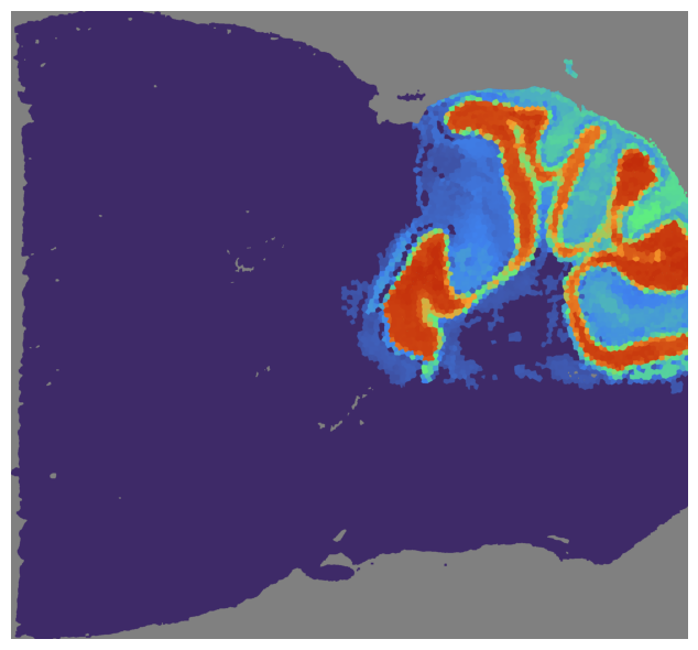
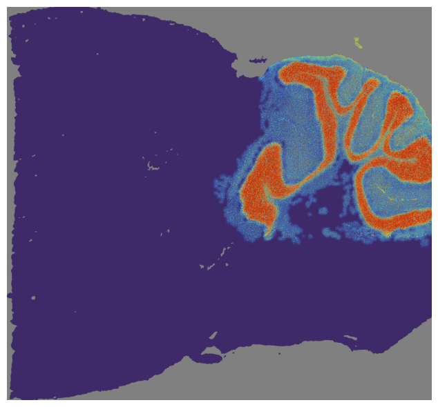
[25]:
# Visualize the SpaHDmap score
mapper.visualize(mouse_posterior, use_score='SpaHDmap', index=2)
*** Visualizing and saving the embeddings of SpaHDmap... ***
Different from the NMF and GCN scores, the SpaHDmap score is a pixel-wise score. For the purposes of reducing storage size and enabling visualization, we save the SpaHDmap scores as images with int type (0-255):
The gray value of each pixel represents the score of that pixel and is stored in
results_path/section_name/SpaHDmap/gray.The color image shows the intensity of the score. It is stored in
results_path/section_name/SpaHDmap/colorafter being scaled by a rate of 4.
[26]:
# Save all SpaHDmap scores into `results_path/section_name/SpaHDmap`
mapper.visualize(use_score='SpaHDmap')
*** Visualizing and saving the embeddings of SpaHDmap... ***
Now NMF, GCN and SpaHDmap scores are available now.
[27]:
mouse_posterior
[27]:
STData object for section: mouse_posterior
Number of spots: 3355
Number of genes: 3000
Image shape: (3, 11607, 11620)
Scale rate: 1
Spot radius: 45
Image type: HE
Available scores: NMF, GCN, VD, SpaHDmap, SpaHDmap_spot
The final metagene matrix is stored in the metagene attribute of the Mapper object.
[28]:
mapper.metagene.head()
[28]:
| Embedding_1 | Embedding_2 | Embedding_3 | Embedding_4 | Embedding_5 | Embedding_6 | Embedding_7 | Embedding_8 | Embedding_9 | Embedding_10 | Embedding_11 | Embedding_12 | Embedding_13 | Embedding_14 | Embedding_15 | Embedding_16 | Embedding_17 | Embedding_18 | Embedding_19 | Embedding_20 | |
|---|---|---|---|---|---|---|---|---|---|---|---|---|---|---|---|---|---|---|---|---|
| Pcp2 | 0.101357 | 0.170434 | 2.171809 | 0.361878 | 0.000000 | 0.071040 | 0.000000 | 0.000000 | 0.000000 | 0.434044 | 0.055079 | 0.000000 | 0.000000 | 0.099606 | 3.027639 | 3.201355 | 0.247909 | 0.000000 | 0.493130 | 0.169384 |
| Mbp | 1.836941 | 3.391119 | 1.954890 | 1.441217 | 2.351305 | 1.096144 | 0.361233 | 2.159111 | 0.524394 | 0.473596 | 0.596884 | 4.252832 | 0.909668 | 1.104496 | 0.398586 | 0.915480 | 0.897189 | 1.217647 | 4.969950 | 1.278716 |
| Nrgn | 1.968724 | 0.050403 | 0.000000 | 0.000000 | 0.000000 | 0.960244 | 1.109673 | 0.031638 | 3.136277 | 0.123370 | 2.272222 | 0.598826 | 3.214096 | 0.000000 | 0.000000 | 0.040291 | 1.719444 | 1.196311 | 0.000000 | 0.000000 |
| Ddn | 0.614909 | 0.000000 | 0.000000 | 0.000000 | 0.000000 | 0.424489 | 0.886830 | 0.007055 | 0.986365 | 0.000000 | 1.764242 | 0.021690 | 1.239175 | 0.000000 | 0.000000 | 0.000000 | 0.000000 | 2.686119 | 0.000000 | 0.086467 |
| Fth1 | 1.875063 | 3.120790 | 2.295356 | 1.472737 | 2.521150 | 2.205889 | 1.648142 | 2.249661 | 1.832261 | 0.462358 | 2.109773 | 3.981107 | 2.165417 | 1.436244 | 1.052056 | 1.483423 | 0.761951 | 2.044789 | 5.382278 | 1.025505 |
Finally, we can save (and load) the STData object using:
[29]:
# Save the STData object
mouse_posterior.save(results_path + 'mouse_posterior.st')
# Load the STData object
# mouse_posterior = hdmap.prepare_stdata(st_path=(results_path + 'mouse_posterior.st'))
5. Downstream analysis
After running SpaHDmap, we can perform downstream analysis, such as clustering and recovering high-resolution gene expression.
[30]:
# Load the STData object
mouse_posterior = hdmap.prepare_stdata(st_path=(results_path + 'mouse_posterior.st'))

# Initialize the SpaHDmap runner with the loaded STData object
mapper = hdmap.Mapper(mouse_posterior, results_path=results_path, rank=rank, verbose=verbose)
*** Loading saved STData from ../experiments//MPBS01/Results_Rank20/mouse_posterior.st ***
*** Preparing the tissue splits and creating pseudo spots... ***
*** Using GPU ***
Clustering
We can perform clustering based on the SpaHDmap score using the cluster function. First, it clusters the spots based on the SpaHDmap score using louvain. Then, it performs K-means clustering based on the embedding of all pixels.
[31]:
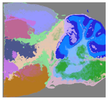
# Cluster pixels based on the SpaHDmap score
mapper.cluster(use_score='SpaHDmap', resolution=0.8, show=True)
*** Performing clustering using SpaHDmap scores... ***
Found 14 clusters for section mouse_posterior
*** Visualizing clustering results for SpaHDmap... ***
The parameters of the cluster function are as follows:
section: the STData object or the name of the sectionuse_score: the score to use for clustering, default is ‘SpaHDmap’n_neighbors: the number of neighbors, default is 50resolution: the resolution for clustering, default is 0.8joint: whether to cluster spots/pixels jointly across sections (if provide multiple sections)format: the format of the clustering results, default is ‘png’show: whether to show the clustering results, default is True
The scaled SpaHDmap pixel clustering results are stored in the clusters attribute of the STData object. Visualization result is saved in results_path/section_name/SpaHDmap/ as image.
[32]:
mouse_posterior.clusters['SpaHDmap']
[32]:
{'spot': array([ 3,  0, 13, ...,  0,  0,  1]),
 'pixel': array([[-1, -1, -1, ..., -1, -1, -1],
        [-1, -1, -1, ..., -1, -1, -1],
        [-1, -1, -1, ..., -1, -1, -1],
        ...,
        [-1, -1, -1, ..., -1, -1, -1],
        [-1, -1, -1, ..., -1, -1, -1],
        [-1, -1, -1, ..., -1, -1, -1]])}
[33]:
mouse_posterior.clusters['SpaHDmap']['pixel'].shape
[33]:
(1999, 2155)
You can also visualize the clustering results using the visualize function, which will save the clustering results in results_path/section_name/SpaHDmap/.
[34]:
# Visualize the clustering results of SpaHDmap
mapper.visualize(target='cluster', use_score='SpaHDmap', format='pdf')
*** Visualizing clustering results for SpaHDmap... ***

You can also cluster the spots based on the NMF score using the same cluster function, just set use_score='NMF'. Visualization results will be saved in results_path/section_name/NMF/ as image.
[35]:
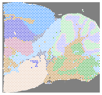
# Cluster spots based on the NMF score
mapper.cluster(use_score='NMF', resolution=0.8, show=True)
*** Performing clustering using NMF scores... ***
Found 11 clusters for section mouse_posterior
*** Visualizing clustering results for NMF... ***
[36]:
mouse_posterior.clusters['NMF']
[36]:
array([0, 1, 5, ..., 1, 1, 3])
Recover high-resolution gene expression
After running SpaHDmap, we can recover and visualize the high-resolution gene expression based on the SpaHDmap score and the metagene matrix. This will save the high-resolution gene expression image in the results_path/section_name/SpaHDmap/genes folder.
[37]:
mouse_posterior.genes[:5]
[37]:
['Pcp2', 'Mbp', 'Nrgn', 'Ddn', 'Fth1']
[38]:
# Load the metagene matrix from the results path
mapper.load_metagene()
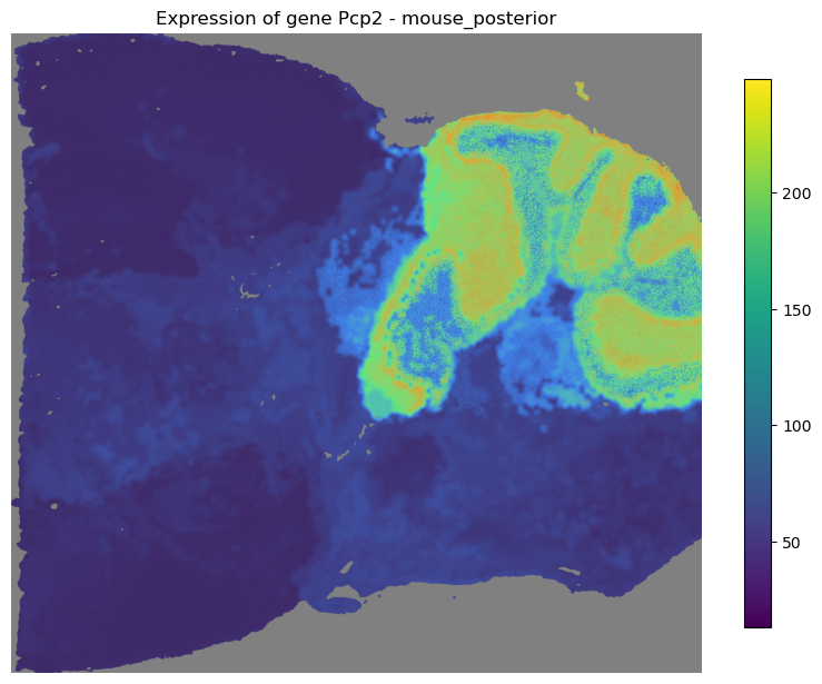
# Recover and visualize the high-resolution gene expression for a specific gene
mapper.recovery(gene=mouse_posterior.genes[:5], use_score='SpaHDmap')
*** Loaded both metagene_NMF and metagene from ../experiments//MPBS01/Results_Rank20/ ***
*** Loaded metagene for transfer learning with 3000 genes ***
*** Updated model nmf_decoder size to (3000, 20) ***
Recovered expression for 5 genes in section mouse_posterior
Recovered gene expressions are stored in the X attribute of the STData object:
[39]:
mouse_posterior.X
[39]:
{'Pcp2': array([[0., 0., 0., ..., 0., 0., 0.],
        [0., 0., 0., ..., 0., 0., 0.],
        [0., 0., 0., ..., 0., 0., 0.],
        ...,
        [0., 0., 0., ..., 0., 0., 0.],
        [0., 0., 0., ..., 0., 0., 0.],
        [0., 0., 0., ..., 0., 0., 0.]]),
 'Mbp': array([[0., 0., 0., ..., 0., 0., 0.],
        [0., 0., 0., ..., 0., 0., 0.],
        [0., 0., 0., ..., 0., 0., 0.],
        ...,
        [0., 0., 0., ..., 0., 0., 0.],
        [0., 0., 0., ..., 0., 0., 0.],
        [0., 0., 0., ..., 0., 0., 0.]]),
 'Nrgn': array([[0., 0., 0., ..., 0., 0., 0.],
        [0., 0., 0., ..., 0., 0., 0.],
        [0., 0., 0., ..., 0., 0., 0.],
        ...,
        [0., 0., 0., ..., 0., 0., 0.],
        [0., 0., 0., ..., 0., 0., 0.],
        [0., 0., 0., ..., 0., 0., 0.]]),
 'Ddn': array([[0., 0., 0., ..., 0., 0., 0.],
        [0., 0., 0., ..., 0., 0., 0.],
        [0., 0., 0., ..., 0., 0., 0.],
        ...,
        [0., 0., 0., ..., 0., 0., 0.],
        [0., 0., 0., ..., 0., 0., 0.],
        [0., 0., 0., ..., 0., 0., 0.]]),
 'Fth1': array([[0., 0., 0., ..., 0., 0., 0.],
        [0., 0., 0., ..., 0., 0., 0.],
        [0., 0., 0., ..., 0., 0., 0.],
        ...,
        [0., 0., 0., ..., 0., 0., 0.],
        [0., 0., 0., ..., 0., 0., 0.],
        [0., 0., 0., ..., 0., 0., 0.]])}
[40]:
mapper.visualize(gene='Pcp2')
*** Visualizing expression of gene Pcp2... ***
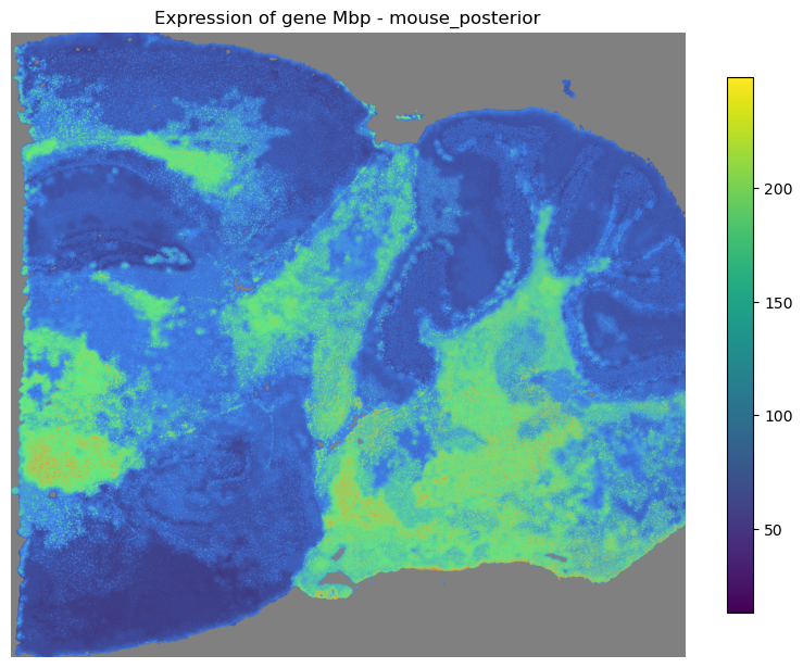
[41]:
mapper.visualize(gene='Mbp')
*** Visualizing expression of gene Mbp... ***