Analysis of IHC-stained imaging data
This tutorial will guide you through the process of running SpaHDmap on IHC stained image ST data. Please see the Step-by-step guide for SpaHDmap workflow tutorial for a more comprehensive introduction to SpaHDmap.
Our example data is a 10X Visium ST dataset MBC-01 sequenced from an adult mouse brain coronal section, comprising three immunohistochemistry (IHC) stained images (DAPI, Anti-GFAP, Anti-NeuN), we will take the IHC image and the spot expression data as input to run SpaHDmap. This data could be downloaded from 10X Genomics or Google Drive.
1. Import necessary libraries
[2]:
import torch
import numpy as np
import scanpy as sc

import SpaHDmap as hdmap
/home/qk/anaconda3/lib/python3.11/importlib/__init__.py:126: FutureWarning: The legacy Dask DataFrame implementation is deprecated and will be removed in a future version. Set the configuration option `dataframe.query-planning` to `True` or None to enable the new Dask Dataframe implementation and silence this warning.
  return _bootstrap._gcd_import(name[level:], package, level)
2. Set the parameters and paths
In this section, we will set the parameters and paths for the SpaHDmap model, including:
Parameters:
rank: the rank / number of components of the NMF modelseed: the random seedverbose: whether to print the log information
Paths:
root_path: the root path of the experimentproject: the name of the projectresults_path: the path to save the results
Parameters settings
By default, we set the rank to 20, the seed to 123, and the verbose to True. You can modify the parameters according to your data.
[3]:
rank = 20
seed = 123
verbose = True

np.random.seed(seed)
torch.manual_seed(seed)
[3]:
<torch._C.Generator at 0x7efc000c7390>
Paths settings
These paths are set with respect to the current directory. You can modify the paths according to your data.
[4]:
root_path = '../experiments/'
project = 'MBC01'

results_path = f'{root_path}/{project}/Results_Rank{rank}/'
3. Load the data and pre-process
The data used in this tutorial is a 10X Visium ST dataset MBC-01 sequenced from an adult mouse brain coronal section, could be downloaded from 10X Genomics or Google Drive.
Next, we download the data from 10X Genomics using scanpy.
[5]:
section_id = 'V1_Adult_Mouse_Brain_Coronal_Section_2'

# Download the data from the 10X website (set include_hires_tiff=True to download the hires image)
adata = sc.datasets.visium_sge(section_id, include_hires_tiff=True)
image_path = adata.uns["spatial"][section_id]["metadata"]["source_image_path"]

# or load the data from a local folder
# adata = sc.read_visium(f'data/{section_id}')
# image_path = f'data/{section_id}/image.tif'
/tmp/ipykernel_1235441/3088077163.py:4: FutureWarning: Use `squidpy.datasets.visium` instead.
  adata = sc.datasets.visium_sge(section_id, include_hires_tiff=True)
/home/qk/anaconda3/lib/python3.11/site-packages/scanpy/datasets/_datasets.py:555: FutureWarning: Use `squidpy.read.visium` instead.
  return read_visium(sample_dir, source_image_path=source_image_path)
/home/qk/anaconda3/lib/python3.11/site-packages/anndata/_core/anndata.py:1820: UserWarning: Variable names are not unique. To make them unique, call `.var_names_make_unique`.
  utils.warn_names_duplicates("var")
/home/qk/anaconda3/lib/python3.11/site-packages/anndata/_core/anndata.py:1820: UserWarning: Variable names are not unique. To make them unique, call `.var_names_make_unique`.
  utils.warn_names_duplicates("var")
Then we can load and preprocess the data.
[6]:
# Load the data from an AnnData object
mouse_cortex = hdmap.prepare_stdata(adata=adata, section_name='mouse_cortex', image_path=image_path)

hdmap.select_svgs(mouse_cortex, n_top_genes=3000)
*** Reading and preparing AnnData for section mouse_cortex ***
Spot radius found in AnnData: 89
Pre-processing gene expression data for 2807 spots and 32285 genes.
Swapping x and y coordinates.
Processing image, seems to be Immunofluorescence image.
Selected 3000 SVGs using moran method.
[7]:
mouse_cortex
[7]:
STData object for section: mouse_cortex
Number of spots: 2807
Number of genes: 3000
Image shape: (3, 24240, 24240)
Scale rate: 1
Spot radius: 89
Image type: Immunofluorescence
Available scores:
4. Run SpaHDmap
Same to case of analyzing H&E-image 10X Visium ST data, we initialize the Mapper object and run SpaHDmap.
[8]:
# Initialize the SpaHDmap runner
mapper = hdmap.Mapper(mouse_cortex, results_path=results_path, verbose=True)

# Run SpaHDmap in one function
mapper.run_SpaHDmap()
*** Preparing the tissue splits and creating pseudo spots... ***
*** Single section detected. Using its 3000 genes. ***
*** The split size is set to 256 pixels. ***
For section mouse_cortex, divide the tissue into 4495 sub-tissues, and create 15000 pseudo spots.
*** Using GPU ***
Step 1: Run NMF
*** Performing NMF... ***
*** Visualizing and saving the embeddings of NMF... ***
Step 2: Pre-train the SpaHDmap model
*** Pre-trained model found at ../experiments//MBC01/Results_Rank20//models//pretrained_model.pth, loading... ***
Step 3: Train the GCN model
*** Performing GCN... ***
*** Training GCN for mouse_cortex... ***
[Iter: 200 / 5000], Loss: 0.018455, Learning rate: 4.985215e-03
[Iter: 400 / 5000], Loss: 0.005902, Learning rate: 4.941093e-03
[Iter: 600 / 5000], Loss: 0.005357, Learning rate: 4.868331e-03
[Iter: 800 / 5000], Loss: 0.005235, Learning rate: 4.768075e-03
[Iter: 1000 / 5000], Loss: 0.005175, Learning rate: 4.641907e-03
[Iter: 1200 / 5000], Loss: 0.005133, Learning rate: 4.491816e-03
[Iter: 1400 / 5000], Loss: 0.005104, Learning rate: 4.320170e-03
[Iter: 1600 / 5000], Loss: 0.005079, Learning rate: 4.129675e-03
[Iter: 1800 / 5000], Loss: 0.005060, Learning rate: 3.923336e-03
[Iter: 2000 / 5000], Loss: 0.005043, Learning rate: 3.704407e-03
[Iter: 2200 / 5000], Loss: 0.005026, Learning rate: 3.476340e-03
[Iter: 2400 / 5000], Loss: 0.005012, Learning rate: 3.242732e-03
[Iter: 2600 / 5000], Loss: 0.005000, Learning rate: 3.007268e-03
[Iter: 2800 / 5000], Loss: 0.004989, Learning rate: 2.773660e-03
[Iter: 3000 / 5000], Loss: 0.004979, Learning rate: 2.545593e-03
[Iter: 3200 / 5000], Loss: 0.004970, Learning rate: 2.326664e-03
[Iter: 3400 / 5000], Loss: 0.004963, Learning rate: 2.120325e-03
[Iter: 3600 / 5000], Loss: 0.004958, Learning rate: 1.929830e-03
[Iter: 3800 / 5000], Loss: 0.004952, Learning rate: 1.758184e-03
[Iter: 4000 / 5000], Loss: 0.004948, Learning rate: 1.608093e-03
[Iter: 4200 / 5000], Loss: 0.004944, Learning rate: 1.481925e-03
[Iter: 4400 / 5000], Loss: 0.004941, Learning rate: 1.381669e-03
[Iter: 4600 / 5000], Loss: 0.004938, Learning rate: 1.308907e-03
[Iter: 4800 / 5000], Loss: 0.004935, Learning rate: 1.264785e-03
[Iter: 5000 / 5000], Loss: 0.004933, Learning rate: 1.250000e-03
*** Visualizing and saving the embeddings of GCN... ***
Step 4: Run Voronoi Diagram
Step 5: Train the SpaHDmap model
*** Trained model found at ../experiments//MBC01/Results_Rank20//models//trained_model.pth, loading... ***
*** Extracting SpaHDmap scores for mouse_cortex... ***
*** Visualizing and saving the embeddings of SpaHDmap... ***
After training, NMF, GCN and SpaHDmap scores are available now.
[9]:
mouse_cortex
[9]:
STData object for section: mouse_cortex
Number of spots: 2807
Number of genes: 3000
Image shape: (3, 24240, 24240)
Scale rate: 1
Spot radius: 89
Image type: Immunofluorescence
Available scores: NMF, GCN, VD, SpaHDmap, SpaHDmap_spot
[10]:
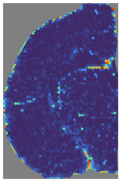
# Visualize the NMF score
mapper.visualize(mouse_cortex, use_score='NMF', index=18)
*** Visualizing and saving the embeddings of NMF... ***
[11]:
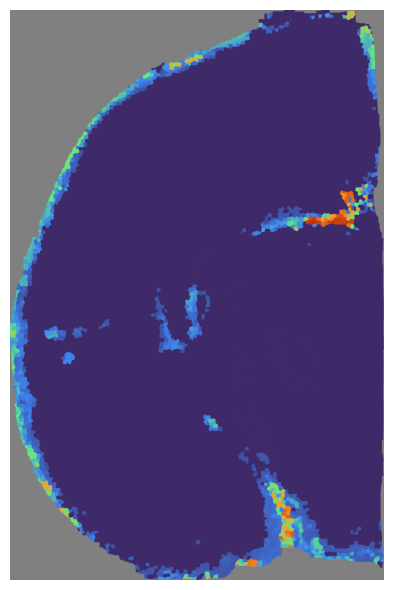
# Visualize the GCN score
mapper.visualize(mouse_cortex, use_score='GCN', index=18)
*** Visualizing and saving the embeddings of GCN... ***
[12]:
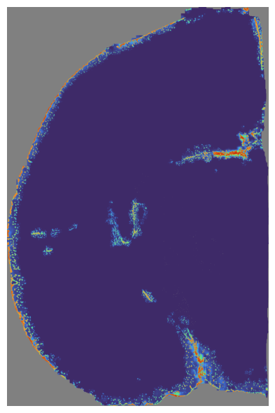
# Visualize the SpaHDmap score
mapper.visualize(mouse_cortex, use_score='SpaHDmap', index=18)
*** Visualizing and saving the embeddings of SpaHDmap... ***
The final metagene matrix is stored in the metagene attribute of the Mapper object.
[13]:
mapper.metagene.head()
[13]:
| Embedding_1 | Embedding_2 | Embedding_3 | Embedding_4 | Embedding_5 | Embedding_6 | Embedding_7 | Embedding_8 | Embedding_9 | Embedding_10 | Embedding_11 | Embedding_12 | Embedding_13 | Embedding_14 | Embedding_15 | Embedding_16 | Embedding_17 | Embedding_18 | Embedding_19 | Embedding_20 | |
|---|---|---|---|---|---|---|---|---|---|---|---|---|---|---|---|---|---|---|---|---|
| Ttr | 0.653175 | 1.833360 | 1.759959 | 0.863542 | 0.635973 | 0.796727 | 1.724082 | 10.820923 | 0.743422 | 0.190398 | 4.749407 | 2.004940 | 2.177563 | 0.056810 | 1.462872 | 0.241082 | 1.046943 | 0.373725 | 0.430738 | 0.987345 |
| Pmch | 0.000000 | 0.134814 | 0.725159 | 4.474846 | 0.000000 | 0.284629 | 0.261490 | 0.288069 | 0.000000 | 0.120419 | 0.147249 | 0.000000 | 0.077970 | 0.000000 | 0.188201 | 0.000000 | 0.181804 | 0.231371 | 0.141038 | 0.608212 |
| Nrgn | 0.920033 | 1.430566 | 1.030315 | 1.025843 | 0.000000 | 2.993280 | 1.609028 | 0.361755 | 0.413251 | 3.758653 | 1.467950 | 0.440135 | 1.782942 | 1.484033 | 2.550623 | 1.692670 | 3.061066 | 2.685826 | 1.156759 | 0.290362 |
| Mbp | 0.261881 | 6.488406 | 3.927031 | 2.893169 | 0.787206 | 1.605631 | 2.251450 | 1.506694 | 0.748659 | 1.882908 | 2.831253 | 3.457766 | 1.625117 | 3.343159 | 2.528405 | 2.594703 | 2.560298 | 1.524600 | 1.682140 | 3.647867 |
| Prkcd | 0.089541 | 0.355763 | 3.671064 | 0.001683 | 0.100243 | 0.286054 | 0.074247 | 0.149027 | 0.076787 | 0.000000 | 0.084735 | 1.190819 | 0.000000 | 0.208558 | 0.000000 | 0.322872 | 0.547407 | 0.000000 | 0.305845 | 0.579738 |
Finally, we can save the STData object:
[14]:
mouse_cortex.save(results_path + 'mouse_cortex.st')